How to create a drop-down list in Excel on Windows and Mac
Adding a drop-down list in Excel is a quick and efficient way to choose predefined data. Here's how to create a drop-down list in Microsoft Excel.
 Koichiko

Implementing a drop-down list in Excel is a quick and efficient way to choose predefined data. In the process, you’re able to save time compared to manually entering such data into a given spreadsheet. Drop-down lists are perfect for several purposes, such as inputting information into a form.
Here's how to create a drop-down list in Microsoft Excel.
Create a drop-down list by manually entering data
There are a few ways to create a drop-down list on Excel. This specific method is the most straightforward and is particularly effective for a Microsoft Excel spreadsheet beginner and for lists that won’t require constant updates.
Step 1: Select the cell in the column where you want to input a drop-down list.
Step 2: Go to the Data tab and select the Data validation button or choose Data validation from the drop-down menu.
Step 3: Pick the Allow menu from the subsequent window that pops up and select List.
Step 4: Within the Source field, enter exactly what you want to be included in the drop-down list. Be sure to apply a comma after each list item.
 Image used with permission by copyright holder
Step 5: Select OK.
The cell you initially selected from step 1 will now have a functioning drop-down list consisting of all the information you entered in step 4.
Create a drop-down list by selecting a range of cells
The most common way to create a drop-down list in Excel with multiple selections is by using a range, which relies on using data from other cells.
Step 1: Choose a column where you want to include the data that will be shown in the associated drop-down list. This can be from the same spreadsheet where the drop-down list will be located, but you can also use a separate spreadsheet (add a new spreadsheet at the bottom). The latter option will naturally make your primary spreadsheet look more tidy, professional, and less cluttered.
Step 2: Type all the data entries into the column, with each entry having its own cell.
 Image used with permission by copyright holder
Step 3: Select the cell where you want the drop-down list to appear.
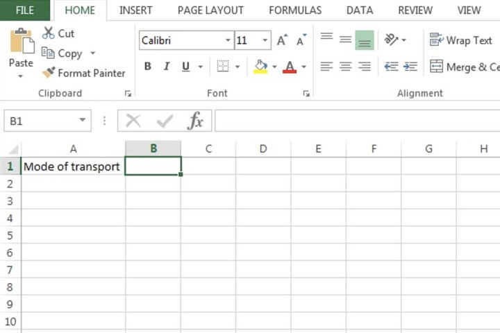 Image used with permission by copyright holder
Step 4: Go to the Data tab and choose Data validation from the drop-down menu.
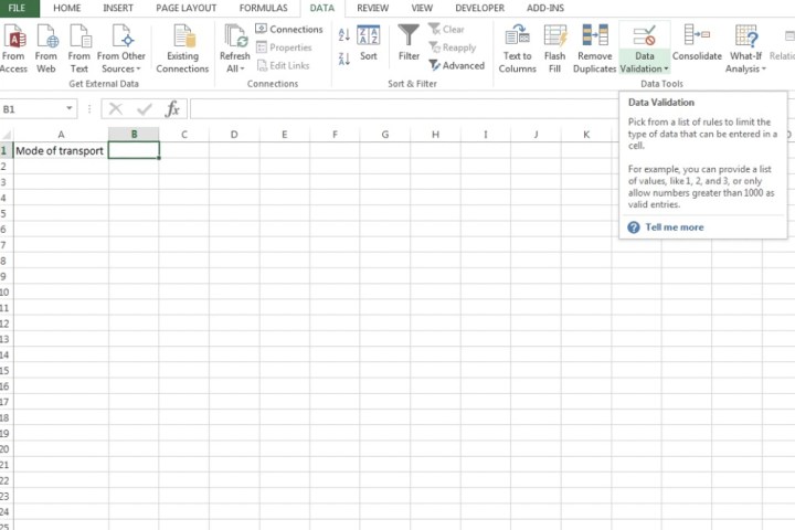 Image used with permission by copyright holder
Step 5: Within the Allow menu, select List. An arrow will be displayed on the edge of the Source field. Select that Arrow.
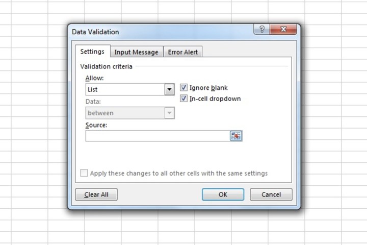 Image used with permission by copyright holder
Step 6: You’ll be taken back to your spreadsheet’s main view. From here, simply select the range of cells by dragging the cursor from the first cell down to wherever your last cell is located.
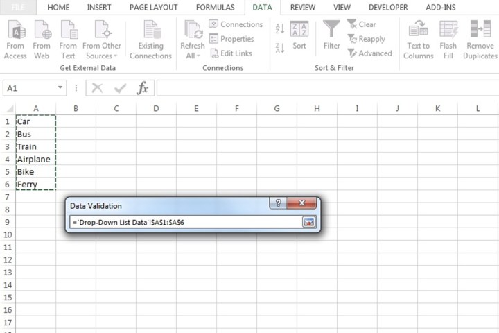 Image used with permission by copyright holder
Step 7: In the Data validation mini pop-up window, select the Arrow button. The Source bar will include the entire cell range that you select in the above steps. Choose OK.
You will now have a drop-down list menu located in the cell you chose from step 3.
 Image used with permission by copyright holder
Display a message when the drop-down list is selected
Once you’ve created your drop-down list, you can make it more accessible by adding an input message.
Step 1: Choose the cell where the drop-down list is located. Then open the Data validation pop-up window once more.
Step 2: Select the Input message tab. Enter a relevant title and the text you want to be displayed when clicking the drop-down list. The text added here is limited to 225 characters.
 Image used with permission by copyright holder
Step 3: Pick "OK" to apply the message.
Display an error alert
Similar to how you can insert a message that describes the purpose of the drop-down list, you can also display an error alert, which can emerge when text or data that’s not found in the list is entered.
Step 1: Select the cell where you created your drop-down. Reopen the Data validation window, select the Error alert tab, and tick the Show error alert after invalid data is entered box.
Enter a custom title and a message. Should the title or text fields be left empty, Excel will apply a default message.
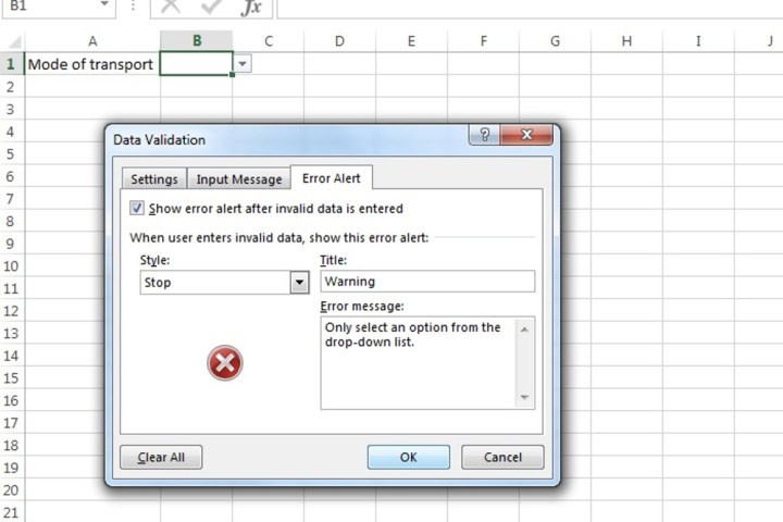 Image used with permission by copyright holder
Step 2: Choose a style from the ones provided, such as Stop (X), and select OK.
Alternatively, if you want a message to pop up that doesn’t prevent individuals from entering invalid data, select either Information or Warning from the Style menu. Both options sport their own design.
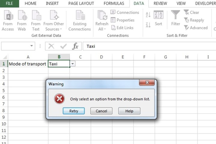 Image used with permission by copyright holder
Protect your drop-down list
To prevent someone from viewing or tampering with the source of the drop-down list’s data, you can lock those cells.
Step 1: Go to the column where your data for the drop-down list is entered. Now select the cells you wish to lock in order to prevent changes from unauthorized sources.
After you’ve selected the area you want to lock, go to the Home tab.
Step 2: Within the Alignment section, select the Small arrow at the bottom right to open the Format cells window. Head to the Protection tab, mark the Locked check box, and select OK.
 Image used with permission by copyright holder
Step 3: Go to the Review tab and select Protect sheet or Protect workbook. Make any adjustments as per your requirements and pick OK.
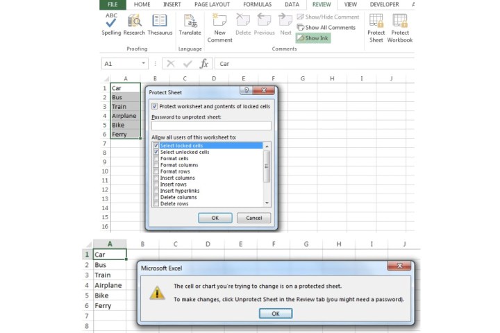 Image used with permission by copyright holder