How to Use The Query Function in Google Sheets

A query function lets you use data commands to shape your data in Google Sheets, making it an important function.

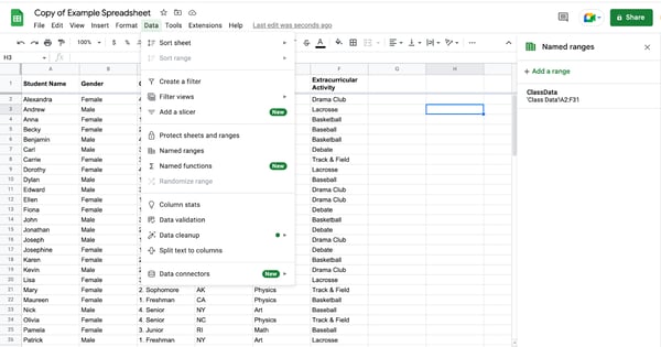
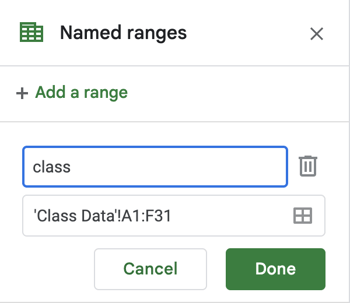
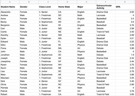
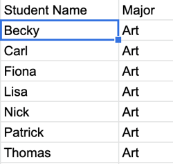
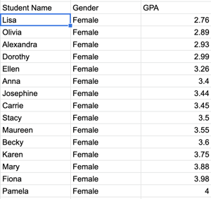
The query function is so helpful because it can replace the work of many other commands and replicate the functionality of pivot tables (a table that lets you group, compare, and summarize larger data sets).

A query may seem complicated or overwhelming if you’re unfamiliar with Google Sheet functions. However, this is not the case, and you can start using the query function right now to filter and quickly look up data in your preferred format.

Table of Contents

What is a query in Google Sheets?

The word query comes from Structured Query Language or SQL, a domain-specific language used in programming to streamline managing large or small data sets.

A query in Google Sheets lets you manipulate and analyze data with a single query formula.

With the query function, you can specify complex conditions for filtering, sorting, and grouping data. You can also use various built-in functions to calculate and transform your data. The output of your query is a new table that only includes the rows and columns that meet the specified conditions.

What syntax should I understand to use the query function?

Here's a basic syntax of a query function in Google Sheets:

Queries are particularly useful when you need to extract a subset of data from a large dataset and when you want to perform complex calculations or transformations on the data.

How to Use Queries in Google Sheets in Three Simple Steps

Create a list of numbered steps on how people can do this. Include screenshots.

1. Name your data.

You will first want to create your first named range, so you don’t have to copy cells every time you want to use them. Using Command for Mac or CTRL for Windows, highlight every cell with data. Click on “Data” and then click “Named Ranges” (pictured below).

You will then name your entire data set, so since this spreadsheet focuses on the names, gender, and extracurricular activities of students, I named it “class.” Be sure not to use any spaces when naming.

You will then enter an empty cell to test your named range. Type in “=query(INSERT NAME OF YOUR DATA)” and see if it highlights all the cells for you (like the picture below).

If you close the parentheses and press “enter,” an identical copy of your data should be generated to the right.

2. Specify what data you want.

Now you can specify which headers you want your query to address. Use the formula below to specify which columns you want to be displayed. I chose columns A and D on my chart so I could see student names and their home states.

After you’ve filled out this formula, go ahead and press enter. If you run into any trouble, make sure you have written it exactly and aren’t missing any commas or parentheses.

You can add any columns you want to the equation by adding a comma and then the letter of the column.

So, had I wanted the student’s name, gender, and home state, I would have written:

=query(class, “select A, B, D”, 1)

3. Get more detailed data.

Say another column includes the student’s GPAs (see below), and we want to know which students have a GPA greater than a 3.0.

You could use the formula below to sort through GPAs and generate a report that includes the students’ names, gender, and GPAs that are above a 3.0.

Say you wanted to know how many students take art as their Extracurricular Activity. You could use this formula to generate that data:

A report (like the one below) would then be generated, so you could know there are seven students in art.

If you want to know which female students have the highest GPAs, you could use the below formula:

And the following report will be generated:

Examples of Queries in Google Sheets

1. Save Time

Pretend you have a giant Google Sheet with the name, gender, role, and age of everyone at a company.

Your boss asks you to give him the name of every person who identifies as a woman at your company so they can be invited to a special women-led conference.

You could spend all afternoon copying over the names and roles of these women, or you could save yourself a lot of time by using a query that generates a report in less than a second, which would look something like this:

=query(staff, “select A, B where B = ‘Female’”, 1)

Here, column “A” is their name, and column “B” is their gender.

2. Get More Accurate Results

Human error is inevitable, especially when you look at the same screen for hours trying to filter data. Every person who’s dealt with large data sets can attest to the struggle of making copy-and-paste errors.

Using queries in google sheets is an exact formula; if you put in the precise terms of data you want, you will generate an accurate report.

3. Reuse the Same Formulas

Once you have a formula you know you use often, you don’t need to write it out over and over again. You can simply click into the report to adjust your formula, or you can save a template of that formula in a separate doc.

For example, if you work in sales and are asked every quarter to present quarterly earnings from the highest to the lowest performer, you can have them add their revenue to a Google Sheet.

Then when it’s time to present, you need only to generate a report using a formula like this:

=query(salespeople, “select A, C order by C asc”, 1)

So “A” would be the name of the salespeople, “C” would be only their revenue for a specific quarter, and “asc” would be from highest to lowest, letting you identify the top performers.

Getting Started

Queries let you analyze and visualize your data in various ways, making it easier to draw insights and make informed decisions.

Have fun experimenting with different query functions to see what you can do with your data!