How-To: Conditional Formatting Based on Another Cell in Google Sheets
Conditional formatting is a feature in Google Sheets in which a cell is formatted in a particular way when certain conditions are met. The formatting can include highlighting, bolding, italicizing – just about any visual changes to the cell.
 Konoly

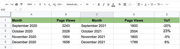
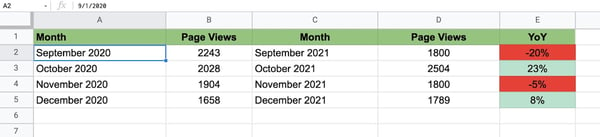
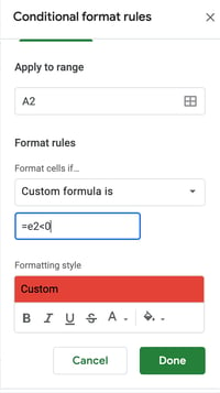
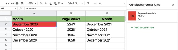
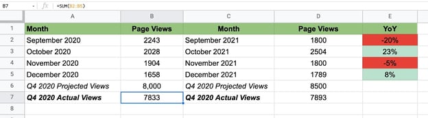
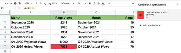
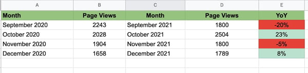
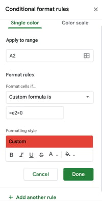
Conditional formatting is a feature in Google Sheets in which a cell is formatted in a particular way when certain conditions are met. The formatting can include highlighting, bolding, italicizing – just about any visual changes to the cell. Just as it can be done for the cell you’re currently in, conditional formatting can also be set based on conditions met in another cell. Let’s dive into how to create this condition based on multiple criteria. To learn how to set conditional formatting, let’s use this workbook as an example. It’s a workbook showing website traffic year over year from Q4 2020 to Q4 2021, with the page views along with the year-over-year percentage change. Here’s what we want to accomplish here: When the percentage change is positive YoY, the cell turns green. When it’s negative, the cell turns red. This makes it easy to get a quick performance overview before diving into the details. Here are the steps to set the conditional formatting. It may automatically default to a standard conditional formatting formula. In this case, open the dropdown menu under "Format cells if…" to select your rules. Options will look as follows: Now that you understand the basics, let’s cover how to use conditional formatting based on other cells. To format based on another cell range, you follow many of the same steps you would for a cell value. What changes is the formula you write. Currently, Google Sheets does not offer a way to use conditional formatting based on the color of another cell. You can only use it based on: To achieve your goal, you’d have to use the condition of the cell to format the other. Let’s use an example. Say you want to format cell A2 (September 2020) to be red and match the color of cell E2 (-20%). There’s no formula that allows you to create a condition based on color. However, you can create a custom formula based on E2’s values. You can say that if cell E2’s values are less than 0, cell A2 turns red. The formula is as follows: = [The other cell] < [value]. In this case, the formula would be =e2<0, as it signifies that cell A2 should turn red if E2’s value is less than 0. With so many functions to play with, Google Sheets can seem daunting. By following these simple steps, you can easily format your cells for quick scanning.![Google Sheets Templates [Free Kit]](https://no-cache.hubspot.com/cta/default/53/e7cd3f82-cab9-4017-b019-ee3fc550e0b5.png)
How Conditional Formatting Works
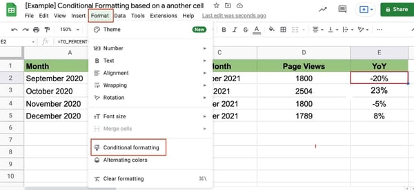
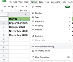
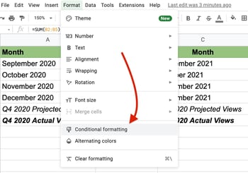
1. Select the cell you want to format, click on "Format" from the navigation bar, then click on "Conditional Formatting."
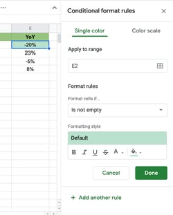
2. While staying in the "Single color" tab, double-check that the cell under "Apply to range" is the cell you want to format.
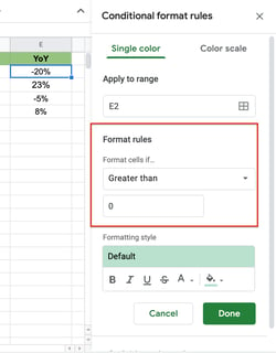
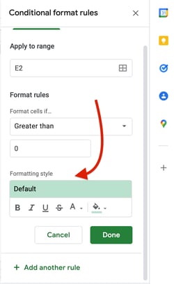
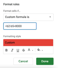
3. Set your format rules.
4. Choose your formatting style, then click "Done."
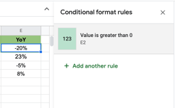
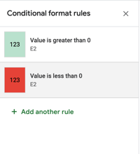
5. Confirm the rule was applied under "Conditional Formatting Rules."
6. Add another rule if needed.
7. Return to cell to view formatting, then drag the cursor to apply to other cells, if needed.
Conditional Formatting Based on Another Cell Value
1. Select the cell you want to format.
2. Click on "Format" in the navigation bar, then select "Conditional Formatting."
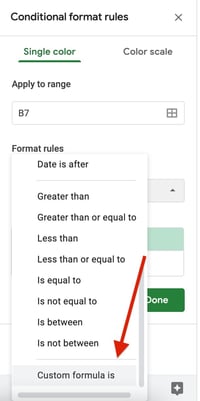
3. Under "Format Rules," select "Custom formula is."
4. Write your formula, then click "Done."
5. Confirm your rule has been applied and check the cell.
Conditional Formatting Based on Another Cell Range
1. Select the cell you want to format.
2. Click on "Format" in the navigation bar, then select "Conditional Formatting."
3. Under "Format Rules," select "Custom formula is."
4. Write your formula using the following format: =value range < [value], select your formatting style, then click "Done."
5. Confirm your rule has been applied and check the cell.
Conditional Formatting Based on Another Cell Not Empty
Google Sheets Conditional Formatting Based on Another Cell Color

Originally published Mar 10, 2022 7:00:00 AM, updated March 10 2022


![Email Automations That Help Turn Tiny Shops Into Mega Marts with Simon Trafford [VIDEO]](https://www.digitalmarketer.com/wp-content/uploads/2022/05/Simon_Thumbnail.jpg)