How To Create a Google Sheets Drop-down Menu

A lot of the data you enter into your Google Sheets tables may be repetitive, like tracking whether an influencer you’ve reached out to for a partnership has agreed to working with you or not.

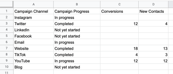
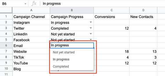
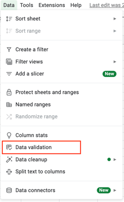
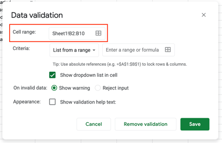
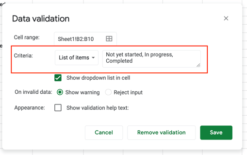
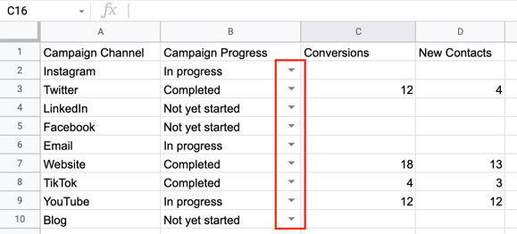
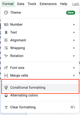
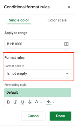
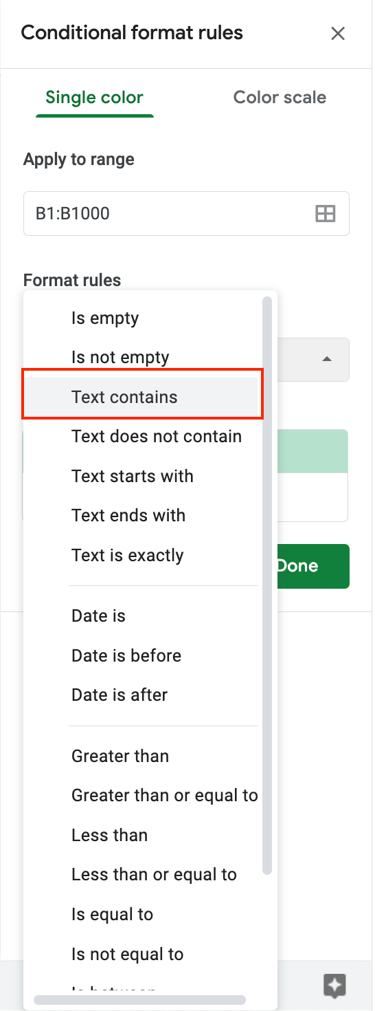
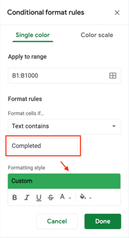
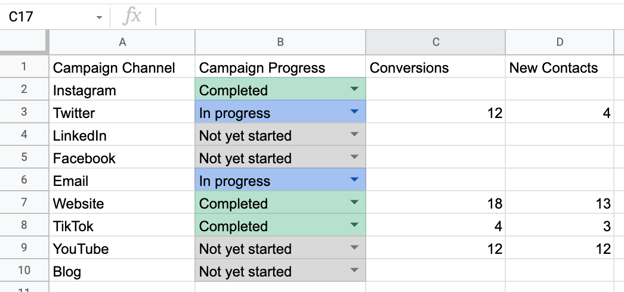
It can get tedious to go in and type each yes or no as time goes on, which is where a critical tool, the drop-down list, becomes your best friend.

In this post, we’ll go over how to add a drop-down list to your own Google Sheets data set to help save time.

How to Add a Drop-down List in Google Sheets

As mentioned above, a drop-down list can help you easily change elements of a cell when the content is repetitive.

The example data set for this walkthrough (as shown in the image below) is tracking the progress of marketing campaigns on different channels and the stage they’re in; not yet started, in progress, or completed. I want to create a drop-down menu so I can easily go in and change the status of the campaign as time goes on.

Before going through the steps, it might be helpful to see what a drop-down menu looks like so you can contextually understand each instruction. The gif below shows a final drop-down menu and how it applies to the sample data set.

Let’s go over how to add a drop-down list to your Sheet.

1. In the toolbar header, click Data.

2. In the drop-down menu, as shown in the image below, select Data validation.

3. In the Data validation dialog box, enter the range of cells you want to have a drop-down menu in Cell range. For this example, I’m entering B2:B10 for cells 2-10 in column B.

4. The next step is to enter the data range that you want to be included in the drop-down menu. Select List of items, and add in your menu values. For this example, this is where I would input Not yet started, In progress, and Complete.

Once you’ve entered your values, click save.

5. Each of your cells should now have a clickable down arrow, as shown in the image below.

For the example table, I can click on each down arrow and change the status of my campaigns as time goes on.

How to Edit a Drop-down List in Google Sheets

If you need to make changes to your drop-down menu, the process is rather simple.

1. In the toolbar header, click Data and then Data validation.

2. In the Data validation dialogue box, simply input the changes you want to make. For example,

If you want to change the items in your drop-down menu, navigate to Criteria, and make your desired changes. If you want to change the column the drop-down menu is in, change the cell numbers in Cell range. If you want to delete your drop-down menu altogether, select the column the menu is currently in and click Remove validation.

Always click save after making all changes.

Color Code a Drop-down List in Google Sheets

Color coding is helpful when it comes to interpreting results at a glance. You can do this with your drop-down list by creating conditional formatting rules, and below we’ll explain how.

1. Select the cells your drop-down menu is in and click Format.

2. Select Conditional formatting from the dialogue box, as shown in the image below.

3. In the Conditional formatting rules sidebar on the right-hand side of your screen, navigate to the Format rules section.

4. In the Format cells if menu, select Text contains…

5. Enter the first element in your drop-down list that you want color-coded. In the image below, I’ve entered Completed as my value and set the color to Green.

6. To set a color for each of your list items, select + Add another rule and repeat step 5 for each value. For my chart, I’ve set In progress to Blue, and Not started to gray.

7. After you set each of your rules, changing the drop-down menu item to a different value will automatically change it to the correct color. For example, if I change Not yet started to In progress, it turns from gray to blue.

Once you’ve created your drop-down menu and color-coded it for easy interpretation, you can continue to track the progress of your different marketing activities and save time while doing so.

Originally published Mar 3, 2022 7:00:00 AM, updated March 03 2022