How to freeze rows and columns in Excel

If you’ve ever worked with an enormous Excel spreadsheet, you’ll know just how daunting all those rows and columns can be. Once you’re over 10 or 15 different values and labels, it can get pretty difficult to hang onto any info you’ve gleaned from these early cells. Fortunately, there’s a simple way to lock those little rectangular boxes of information.

The name of the game is “freezing,” and the execution is about as surface-level as the word. You freeze specific rows and columns, so when you’re scrolling through, these cells remain stationary on the page.

Here's our step-by-step guide to teach you how to start freezing today!

How to freeze a row in Excel

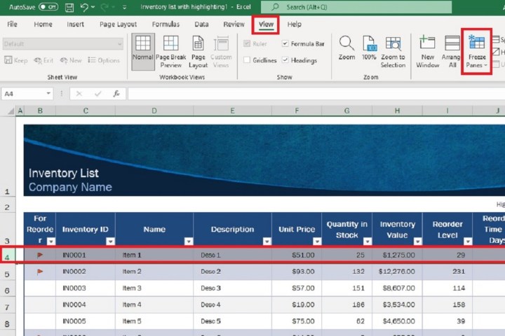
Step 1: Pick out the row or rows you want to freeze. These will be the rows that will stay with you as you scroll through the spreadsheet. Select the row immediately below the row you want to freeze. So if you want to freeze rows 1-3, you need to select row 4.

Step 2: Then select the View tab from the ribbon menu at the top of the screen.

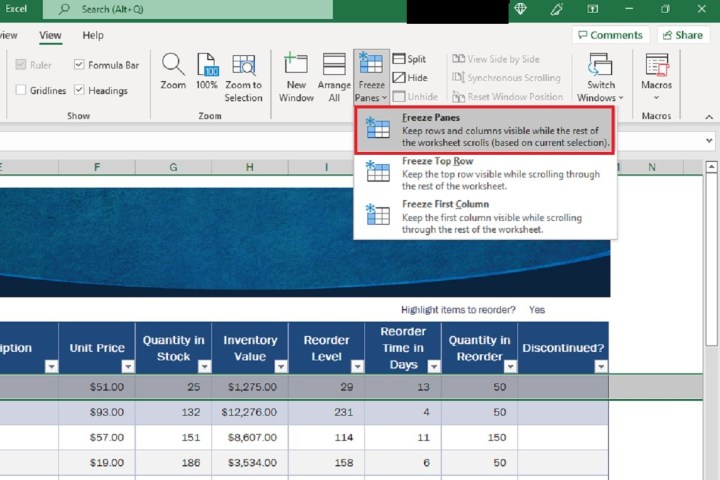
Step 3: From the drop-down menu that appears, select Freeze Panes.

Alternatively, if all you want to do is freeze the top row of your spreadsheet, you don't have to select any rows beforehand. You can just click on the View tab and then Freeze Panes > Freeze Top Row.

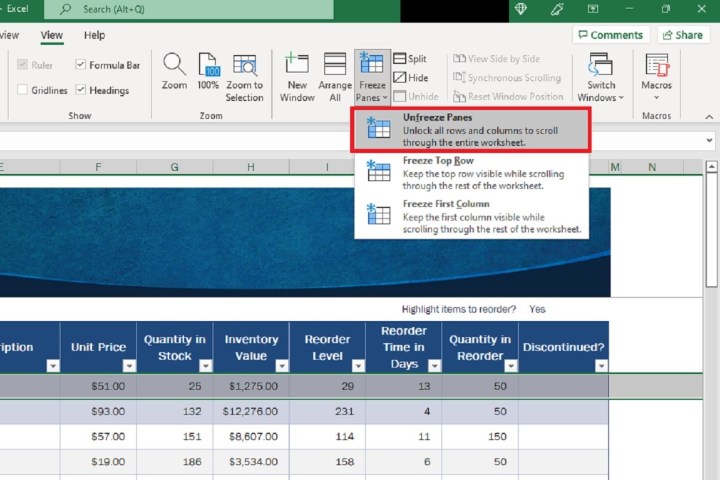
Step 4: To unfreeze your frozen rows: Go to the View tab again, select Freeze Panes, and then choose Unfreeze Panes from the drop-down menu.

How to freeze a column in Excel

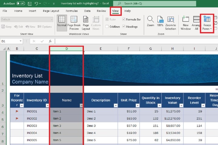
Step 1: Pick the columns you want to freeze. Then select the column that is immediately to the right of the column or columns you want to freeze. For example, if you need to freeze columns A, B, and C, you should select column D.

Step 2: Then select the View tab from the ribbon menu at the top of the screen. Then choose Freeze Panes.

Step 3: From the drop down menu that appears, select Freeze Panes.

Alternatively, if all you want to do is freeze the first column of your spreadsheet, you can just click on the View tab, and then select Freeze Panes > Freeze First Column.

Step 4: To unfreeze your frozen columns, just click on the View tab, and select Freeze Panes > Unfreeze Panes.

Freezing rows and columns with keyboard shortcuts

You can also freeze Excel rows and columns with keyboard shortcuts. Here’s a small list of the most popular commands:

Step 1: Freeze both rows and columns: Press Alt+W+F+F, with each key tap taking place after the last. Once you’ve selected a cell in Excel, this command freezes the rows and columns before the highlighted cell.

Step 2: Freeze the top row: Press Alt+W+F+R. Regardless of the cell that’s selected, this command will always freeze the first row in your spreadsheet.

Step 3: Freeze the first column: Press Alt+W+F+C. Regardless of the cell that’s selected, this command will always freeze the first (leftmost) column in your spreadsheet.

How do you freeze rows and columns in Google Sheets?

Similar to Excel, Google’s own spreadsheet software has freeze-unfreeze options for you to mess around with. Here’s how to access these settings:

Step 1: Open a new spreadsheet in Google Sheets.

Step 2: Choose the row or column you’d like to freeze or unfreeze. Then, click View > Freeze at the top of the page.

Step 3: Now just select how many rows or columns you’d like to freeze. To unfreeze, click View > Freeze > No rows or No columns.

How do you freeze rows and columns in MacOS Numbers?

While Apple’s first-party spreadsheet software doesn’t actually have the same kind of freeze-unfreeze capabilities as Excel or Google Sheets, you can still freeze header rows, header columns, or both. Here’s how:

Step 1: Open a Numbers spreadsheet and click any area of the table. Then, click Table at the top of the page.

Step 2: Choose Freeze Header Rows, Freeze Header Columns, or both. You can also select Header Rows and Header Columns to choose how many rows or columns to freeze.

Editors' Note: Article was checked on March 1, 2023, and confirmed that the steps and information included are still accurate.

Editors' Recommendations